Naive Bayes is one of the fastest methods of classification. Naive Bayes classifier is successfully used in various applications such as spam filtering, text classification, sentiment analysis, and recommender systems. It uses Bayes theorem of probability for prediction of an unknown class.
Naive Bayes is a statistical classification technique based on Bayes Theorem. It is one of the simplest supervised learning algorithms. Naive Bayes classifier is the fast, accurate and reliable algorithm. Naive Bayes classifiers have high accuracy and speed on large datasets.
Naive Bayes classifier assumes that the effect of a particular feature in a class is independent of other features. For example, a loan applicant is desirable or not depending on his/her income, previous loan and transaction history, age, and location. Even if these features are interdependent, these features are still considered independently. This assumption simplifies computation, and that's why it is considered as naive. This assumption is called class conditional independence.
The formula we us is as follows
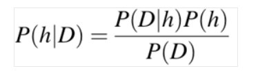
Where the variables are
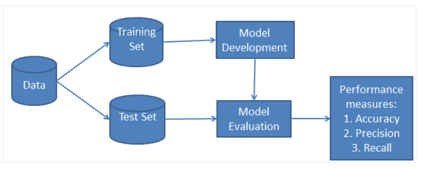
https://www.datacamp.com/tutorial/naive-bayes-scikit-learn I used this course to learn how to do Naive Bayes with scilearn. I am using a loan dataset from kaggle to try to find a way to automate my loan acceptance process. I know this will be a classification problem since my target variable is the status of the loan acceptance. The following variables I will use include:
from sklearn.linear_model import LogisticRegression

from sklearn.model_selection import train_test_split

from sklearn import metrics

import pandas as pd

import numpy as np

import matplotlib.pyplot as plt

import seaborn as sns

import warnings
warnings.filterwarnings('ignore')
dataset = pd.read_csv('loan_data.csv')
dataset = dataset[['CoapplicantIncome', 'ApplicantIncome', 'Credit_Score', 'Loan_Status']]
dataset
| CoapplicantIncome | ApplicantIncome | Credit_Score | Loan_Status | |
|---|---|---|---|---|
| 0 | 1508.0 | 4583 | 37 | N |
| 1 | 0.0 | 3000 | 64 | Y |
| 2 | 2358.0 | 15 | 89 | Y |
| 3 | 0.0 | 6000 | 48 | Y |
| 4 | 1516.0 | 2333 | 65 | Y |
| ... | ... | ... | ... | ... |
| 366 | 0.0 | 5703 | 68 | Y |
| 367 | 1950.0 | 3232 | 79 | Y |
| 368 | 0.0 | 2900 | 90 | Y |
| 369 | 0.0 | 4106 | 93 | Y |
| 370 | 0.0 | 4583 | 6 | N |
371 rows × 4 columns
A simple Naive-Bayes classifier can be created to analyze the relationship between our predictors and target variable. Depending on our results, there are other model options to explore. Sklearn will do most of the computing for us. Converting the columns to arrays is essential before creating the model. The GaussianNB() function will create the model once the data cleaning is complete.
# Importing the necessary packages
import sklearn
from sklearn.datasets import load_breast_cancer


# Loading the dataset and organizing the data
DataSet = load_breast_cancer()
labelnames = DataSet['target_names']
labels = DataSet['target']
featurenames = DataSet['feature_names']
features = DataSet['data']

features = dataset[["CoapplicantIncome", "ApplicantIncome", "Credit_Score"]].to_numpy()
labels = dataset[["Loan_Status"]].to_numpy()


# Organizing dataset into training and testing set
# by using train_test_split() function

train, test, train_labels, test_labels = train_test_split(features,labels,test_size = 0.30, random_state = 300)

# Model evaluation by using Naïve Bayes algorithm.
from sklearn.naive_bayes import GaussianNB

# Let's initializing the model:
NBclassifier = GaussianNB()

# Train the model:
NBmodel = NBclassifier.fit(train, train_labels)
# Making predictions by using pred() function:
NBpreds = NBclassifier.predict(test)
print("The predictions are:\n", NBpreds[:15])

# Finding accuracy of our Naive Bayes classifier:
from sklearn.metrics import accuracy_score
print("Accuracy of our classifier is:", accuracy_score(test_labels, NBpreds))
The predictions are:
 ['Y' 'Y' 'Y' 'Y' 'Y' 'Y' 'Y' 'N' 'Y' 'N' 'N' 'Y' 'Y' 'Y' 'Y']
Accuracy of our classifier is: 0.9642857142857143
We can use 2 methods to better analyze the results. The confusion_matrix() function and accuracy_score() function help us analyze.
from sklearn.metrics import confusion_matrix, accuracy_score
cm = confusion_matrix(test_labels, NBpreds)
print(cm)
accuracy_score(test_labels,NBpreds)
[[24  3]
 [ 1 84]]
0.9642857142857143
My confusion matrix states that there are 24 true positives compared to 3 false. There are 84 true negatives compared to 1 false. This means only one person got rejected that was actually supposed to be accepted. That is good but on the other hand, 3 people got accepted that were not supposed to. This leads us to an overall accuracy of 96.4%. This is a little bit deceiving because it a direct correlation of there being more entries on declined applications. This model mostly automates the process of going through applicants that will get declined but the approved applications should still be double checked. Adding more parameters or finding more data could conribute to autmoating accepted applications as well.
I can now confirm the accuracy is high, but would like to create a visualization to see each point individually.
from sklearn.datasets import make_classification
# Importing libraries
from sklearn.datasets import make_classification
import matplotlib.pyplot as plt

# Creating the classification dataset with one informative feature and one cluster per class
nb_samples = 300
X, Y = make_classification(n_samples=nb_samples, n_features=2, n_informative=2, n_redundant=0)

# Plotting the dataset
plt.figure(figsize=(7.50, 3.50))
plt.subplots_adjust(bottom=0.05, top=0.9, left=0.05, right=0.95)
plt.subplot(111)
plt.scatter(X[:, 0], X[:, 1], marker="o", c=Y, s=40, edgecolor="k")
plt.show()

This visualization shows there is a clear separation of classes and why our accuracy was high. I accomplised the goal of automatically declining unapproved applications but still would like to find a better way to classifier approved ones. An SVM, decision tree, or logistic regression could help me in this task.