One of the earliest Monte Carlo simulations was conducted by mathematician and naturalist Buffon, in 1777. He tossed a coin 2,048 times and recorded the results, to study the distribution of the possible outcomes

John von Neumann (left) and Stanislaw Ulam(right) invented the Monte Carlo simulation, or the Monte Carlo method, in the 1940s. They named it after the famous gambling location in Monaco because the method shares the same random characteristic as a roulette game. Both of these Scientists later went to work on the Manhatten Project.

For a mathematician, the height of a population would be called a random variable, because the height among people making up this population varies randomly. We generally denote random variables with upper case letters. The letter X is commonly used.
In statistics, the elements making up that population, which as suggested before are random, are denoted with a lower capital letter, generally as well. For example, if we write , this would denote the height (which is random) of the second person in the collection of samples. All these 's can also be seen as the possible outcomes of the random variable X. If we call X this random variable (the population height), we can express the concept of approximating the average adult population height from a sample with the following pseudo-mathematical formula:
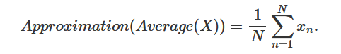
Which you can read as, the approximation of the average value of the random variable X, (the height of the adult population of a given country), is equal to the sum (the sign) of the height of N adults randomly chosen from that population (the samples), divided by the number N (the sample size). This, in essence, is what we call a Monte Carlo approximation. It consists of approximating some property of a very large number of things, by averaging the value of that property for N of these things chosen randomly among all the others. You can also say that Monte Carlo approximation, is a method for approximating things using samples. What we will learn in the next chapters, is that the things which need approximating are called in mathematics expectations (more on this soon). As mentioned before the height of the adult population of a given country can be seen as a random variable X. However, note that its average value (which you get by averaging all the heights for example of each person making up the population, where each one of these numbers is also a random number) is unique (to avoid confusion with the sample size which is usually denoted with the letter N, we will use M to denote the size of the entire population):
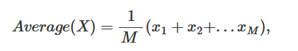
where the corresponds to the height of each person making up the entire population as suggested before (if we were to take an example). In statistics, the average of the random variable X is called an expectation and is written E(X).
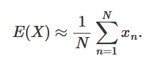
To summarize, Monte Carlo approximation (which is one of the MC methods) is a technique to approximate the expectation of random variables, using samples. It can be defined mathematically with the following formula:
The following shows a simple example with Python similar to Buffon's experiment 300 years ago.
import random
import math
import numpy as np
import pandas as pd
from pandas_datareader import data
import matplotlib.pyplot as plt
import seaborn as sns
from scipy.stats import norm
import warnings
warnings.filterwarnings('ignore')
The next 2 functions are publicly available and will help with the simulation
def coin_flip():
    return random.randint(0,1)

list1 = []
def monte_carlo(n):
    results = 0
    for i in range(n):
        flip_result = coin_flip()
        results = results + flip_result


        prob_value = results / (i+1)

        list1.append(prob_value)


        plt.axhline(y=.5, color = 'r', linestyle = '-')
        plt.xlabel("iterations")
        plt.ylabel("Probability")
        plt.plot(list1)


    return results/n
This function will use only one parameter which will be the number of simulations. The probability starts off volatile but then settles close to .5 after many simulations.
answer = monte_carlo(5000)
print("Final Probability :",answer)
Final Probability : 0.5012

import yfinance as yf

def get_yahoo_data(ticker, start, end):
    data = yf.download(ticker, start=start, end=end)
    return data['Adj Close']
def monte_carlo_simulation(ticker, start, end, num_simulations):
    # Get historical data
    prices = get_yahoo_data(ticker, start, end)

    # Calculate daily returns
    daily_returns = prices.pct_change().dropna()

    # Calculate mean and standard deviation of daily returns
    mean_return = daily_returns.mean()
    std_dev = daily_returns.std()

    # Generate random numbers based on normal distribution
    simulations = np.random.normal(loc=mean_return, scale=std_dev, size=(num_simulations, len(prices)))

    # Calculate simulated prices
    simulated_prices = prices.iloc[-1] * (1 + simulations).cumprod(axis=1)

    # Visualize results
    plt.figure(figsize=(10, 6))
    plt.plot(simulated_prices.T, alpha=0.1)
    plt.title('Monte Carlo Simulation for {}'.format(ticker))
    plt.xlabel('Days')
    plt.ylabel('Price')
    plt.show()
I will conduct multiple experiments and see how each experiment affects our model. Nvidia is one of the highest growing stocks right now so this model should show high future growth with some of the simulations getting out of hand.
# Define stock ticker and time period
ticker = 'NVDA'
start_date = '2020-01-01'
end_date = '2024-01-25'

# Number of simulations
num_simulations = 12

# Perform Monte Carlo simulation
monte_carlo_simulation(ticker, start_date, end_date, num_simulations)
[*********************100%%**********************] 1 of 1 completed

MKTX is a lower performing stock and we can expect the simulations to not show much growth. Some simulations should show a decline. This example shows how we can use the time parameter as well to yield different results.
# Define stock ticker and time period
ticker = 'MKTX'
start_date = '2020-01-01'
end_date = '2024-01-25'

# Number of simulations
num_simulations = 12

# Perform Monte Carlo simulation
monte_carlo_simulation(ticker, start_date, end_date, num_simulations)
[*********************100%%**********************] 1 of 1 completed

This last example shows how more simulations can change our experiment. It can make the graph harder to interpret because we have more opportunities of a simulation being an outlier.