1 - Statistics (Descriptive and Inferential):
Terminologies In Statistics – Statistics For Data Science
One should be aware of a few key statistical terminologies while dealing with Statistics for Data Science. I’ve discussed these terminologies below:
- Population is the set of sources from which data has to be collected.
- A Sample is a subset of the Population
- A Variable is any characteristics, number, or quantity that can be measured or counted. A variable may also be called a data item.
- Also known as a statistical model, A statistical Parameter or population parameter is a quantity that indexes a family of probability distributions. For example, the mean, median, etc of a population.
Categories In Statistics
- Quantitative Analysis: Quantitative Analysis or the Statistical Analysis is the science of collecting and interpreting data with numbers and graphs to identify patterns and trends.
- Qualitative Analysis: Qualitative or Non-Statistical Analysis gives generic information and uses text, sound and other forms of media to do so.
For example, if I want a purchase a coffee from Starbucks, it is available in Short, Tall and Grande. This is an example of Qualitative Analysis. But if a store sells 70 regular coffees a week, it is Quantitative Analysis because we have a number representing the coffees sold per week.
Although the purpose of both these analyses is to provide results, Quantitative analysis provides a clearer picture hence making it crucial in analytics. Topics about Descriptive Statistics:
Descriptive Statistics
Descriptive Statistics uses the data to provide descriptions of the population, either through numerical calculations or graphs or tables.
Descriptive Statistics helps organize data and focuses on the characteristics of data providing parameters.
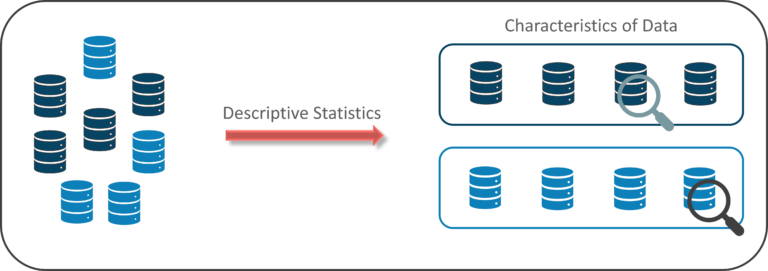
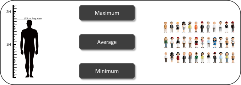
Suppose you want to study the average height of students in a classroom, in descriptive statistics you would record the heights of all students in the class and then you would find out the maximum, minimum and average height of the class.
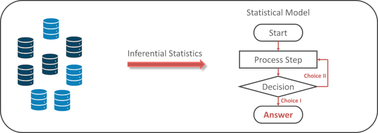
Inferential Statistics Inferential Statistics makes inferences and predictions about a population based on a sample of data taken from the population in question.
Inferential statistics generalizes a large data set and applies probability to arrive at a conclusion. It allows you to infer parameters of the population based on sample stats and build models on it.
Inferential Statistics - Course Curriculum Data Science Training Masters Program
Inferential Statistics –
So, if we consider the same example of finding the average height of students in a class, in Inferential Statistics, you will take a sample set of the class, which is basically a few people from the entire class. You already have had grouped the class into tall, average and short. In this method, you basically build a statistical model and expand it for the entire population in the class.
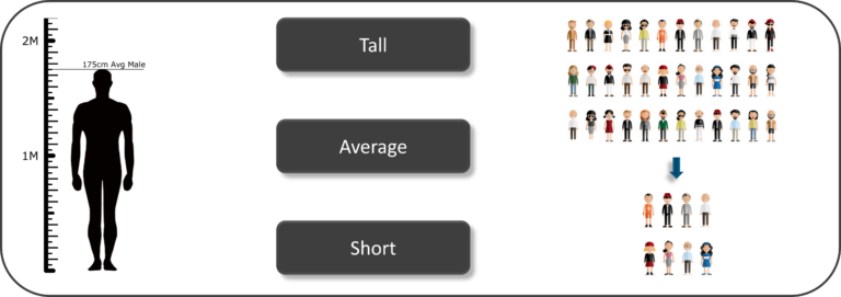
Now let’s focus our attention on Descriptive Statistics and see how it can be used to solve analytical problems. Understanding Descriptive Analysis
When we try to represent data in the form of graphs, like histograms, line plots, etc. the data is represented based on some kind of central tendency. Central tendency measures like, mean, median, or measures of the spread, etc are used for statistical analysis. To better understand Statistics lets discuss the different measures in Statistics with the help of an example.

Here is a sample data set of cars containing the variables:
- Cars
- Mileage per Gallon (mpg)
- Cylinder Type (cyl)
- Displacement (disp)
- Horse Power (hp)
- Real Axle Ratio (drat).
Before we move any further, let’s define the main Measures of the Center or Measures of Central tendency. Measures Of The Center
Mean: Measure of average of all the values in a sample is called Mean.
Median: Measure of the central value of the sample set is called Median.
Mode: The value most recurrent in the sample set is known as Mode.
Using descriptive Analysis, you can analyse each of the variables in the sample data set for mean, standard deviation, minimum and maximum.
If we want to find out the mean or average horsepower of the cars among the population of cars, we will check and calculate the average of all values. In this case, we’ll take the sum of the Horse Power of each car, divided by the total number of cars:
Mean = (110+110+93+96+90+110+110+110)/8 = 103.625
If we want to find out the center value of mpg among the population of cars, we will arrange the mpg values in ascending or descending order and choose the middle value. In this case, we have 8 values which is an even entry. Hence we must take the average of the two middle values.
The mpg for 8 cars: 21,21,21.3,22.8,23,23,23,23 Median = (22.8+23 )/2 = 22.9
If we want to find out the most common type of cylinder among the population of cars, we will check the value which is repeated most number of times. Here we can see that the cylinders come in two values, 4 and 6. Take a look at the data set, you can see that the most recurring value is 6. Hence 6 is our Mode.
Measures Of The Spread
Just like the measure of center, we also have measures of the spread, which comprises of the following measures:
Range: It is the given measure of how spread apart the values in a data set are.
Inter Quartile Range (IQR): It is the measure of variability, based on dividing a data set into quartiles.
Variance: It describes how much a random variable differs from its expected value. It entails computing squares of deviations.
    Deviation is the difference between each element from the mean.
    Population Variance is the average of squared deviations
    Sample Variance is the average of squared differences from the mean
Standard Deviation: It is the measure of the dispersion of a set of data from its mean.
Understanding Inferential Analysis
Statisticians use hypothesis testing to formally check whether the hypothesis is accepted or rejected. Hypothesis testing is an Inferential Statistical technique used to determine whether there is enough evidence in a data sample to infer that a certain condition holds true for an entire population.
To under the characteristics of a general population, we take a random sample and analyze the properties of the sample. We test whether or not the identified conclusion represents the population accurately and finally we interpret their results. Whether or not to accept the hypothesis depends upon the percentage value that we get from the hypothesis.
2) IQR, percentiles
What is the Interquartile Range (IQR)?
The interquartile range (IQR) measures the spread of the middle half of your data. It is the range for the middle 50% of your sample. Use the IQR to assess the variability where most of your values lie. Larger values indicate that the central portion of your data spread out further. Conversely, smaller values show that the middle values cluster more tightly.
In this post, learn what the interquartile range means and the many ways to use it! I’ll show you how to find the interquartile range, use it to measure variability, graph it in boxplots to assess distribution properties, use it to identify outliers, and test whether your data are normally distributed.
The interquartile range is one of several measures of variability. To learn about the others and how the IQR compares, read my post, Measures of Variability. Interquartile Range Definition
To visualize the interquartile range, imagine dividing your data into quarters. Statisticians refer to these quarters as quartiles and label them from low to high as Q1, Q2, Q3, and Q4. The lowest quartile (Q1) covers the smallest quarter of values in your dataset. The upper quartile (Q4) comprises the highest quarter of values. The interquartile range is the middle half of the data that lies between the upper and lower quartiles. In other words, the interquartile range includes the 50% of data points that are above Q1 and below Q4. The IQR is the red area in the graph below, containing Q2 and Q3 (not labeled).
3) Std deviation and Variance
Standard Deviation
The Standard Deviation is a measure of how spread out numbers are.
Its symbol is σ (the greek letter sigma)
The formula is easy: it is the square root of the Variance. So now you ask, "What is the Variance?" Variance
The Variance is defined as:
The average of the squared differences from the Mean.
To calculate the variance follow these steps:
- Work out the Mean (the simple average of the numbers)
- Then for each number: subtract the Mean and square the result (the squared difference).
- Then work out the average of those squared differences. (Why Square?)
4) and 5) Normal Distribution, Z-statistics and T-statistics
See Experimental Design Guide
6) correlation and linear regression
Covariance
If 2 quantities have a positive covariance, they increase/decrease together. For example, salary has a positive covariance with respect to no. of hours worked. If a person works for more hours, their salary is higher. Example of a negative co-variance would be the no. of hours you practice a game w.r.t the chances of losing the game. The more you practice, the lesser are your chances of losing the game.
Directional relationship between two variables.
When we calculate the time taken for a ball to reach the ground when thrown from a fixed height, we know that the mass does not affect the time taken. Hence mass has zero covariance to the time taken. Now, if air resistance is high, the ball takes longer to fall. More the resistance, more the time it takes. This is a positive covariance. If the ball is thrown with more force, lesser the time it takes to reach the ground. This is a negative covariance. Correlation
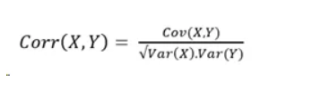
Correlation shows us both, the direction and magnitude of how two quantities vary with each other. Eg. No. of products bought from a store would have a stronger correlation to the profits than the no. of advertisements would have to the profits.
Hence, Corr(no. of products,profit)>Corr(ads posted,profit).
One must note that both will be positive correlations, with ‘no. of products’ having a higher positive value.
This is used in feature selection to determine which feature affects the result the most.
A correlation of +1 indicates a perfect positive correlation.
A correlation of -1 indicates a perfect negative correlation.
A correlation of 0 indicates that there is no relationship between the different variables (mass of a ball does not affect time taken to fall).
Values between -1 and 1 denote the strength of the correlation.
Lets take a look at the formulae: Variance
A random variable is compared against itself.
Var(X) = E(X.X) — E(X).E(X) Covariance
Two random variables compared against each other.
Cov(X,Y) = E(X.Y) — E(X).E(Y) Correlation
Normalized
