Predicting Diabetes Using Logistic Regression and SciKit

The following analysis will use data from a hospital that tracks the prevalance of diabetes in patients with suspected contributing factors measured as well. My goal is to help the patients prevent diabetes. I am going to create a logistic regression model so I can predict when a patient is on track to enter the diabetes range.

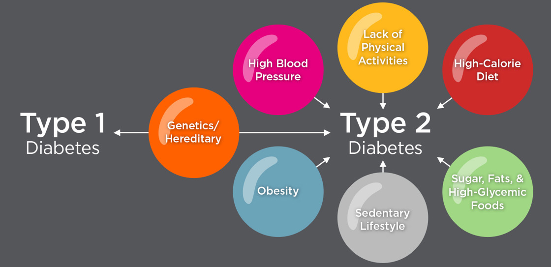
As the graphic shows, type 2 diabetes is a preventable disease since most of the contributing factors can be controlled. The predictor varaibles in our dataset are:

• Pregnancies
• Glucose
• BloodPressure
• SkinThickness
• Insulin
• BMI
• DiabetesPedigreeFunction - calculates diabetes likelihood depending on the subject's age and his/her diabetic family history
• Age
• Outcome - 1 if the patient has diabetes and 0 if not

I will create multiple models and visualizations to find our best predictors for diabetes. Before I do this I need to prepare the data.

Step 1- Import packages and prepare data.

To clean the data I will use pandas, numpy and base python. I will use Scikit to create the models and matplotlib/seaborn to visualize.

import warnings
from sklearn.linear_model import LogisticRegression 
from sklearn.model_selection import train_test_split 
from sklearn import metrics 
import pandas as pd 
import numpy as np 
import matplotlib.pyplot as plt 
import seaborn as sns 

Let' take a look at our data.

# load dataset 
warnings.filterwarnings('ignore')
diab_df = pd.read_csv("Hospital.csv") 

diab_df.head()

	Pregnancies	Glucose	BloodPressure	SkinThickness	Insulin	BMI	DiabetesPedigreeFunction	Age	Outcome
0	6	148	72	35	0	33.6	0.627	50	1
1	1	85	66	29	0	26.6	0.351	31	0
2	8	183	64	0	0	23.3	0.672	32	1
3	1	89	66	23	94	28.1	0.167	21	0
4	0	137	40	35	168	43.1	2.288	33	1

It is clear that outcome will be our target variable. The other columns will all be our features. Next, I will seperate the features from the target, as well as seperating out testing and training data.

Step 2- Train Initial Model

I will start with a single response predictor. The Diabetes Pedigree Function is supposed to be a good predictor for diabetes so I will start with it.

diab_cols = ['DiabetesPedigreeFunction'] 

X = diab_df[diab_cols]# Features 

y = diab_df.Outcome # Target variable 


X_train,X_test,y_train,y_test=train_test_split(X,y,test_size=0.25,random_state=0) 


# instantiate the model 

logreg =  LogisticRegression(solver='liblinear') 

# fit the model with data 

logreg.fit(X_train,y_train) 

# predicting 

y_pred=logreg.predict(X_test) 

y_pred 

cnf_matrix = metrics.confusion_matrix(y_test, y_pred) 

cnf_matrix 

array([[124,   6],
       [ 55,   7]], dtype=int64)

Step 3- Adjust Feature Selection

For detecting a patient whos is close to or has a positive case of diabetes, this method works great with over 95 % accuracy. However, the number of false positives is alarmingly high and would not be accepted. I am going to need to use a different variable or use multiple.

#split dataset in features and target variable 

diab_cols = ['BMI', 'Age','DiabetesPedigreeFunction'] 

X = diab_df[diab_cols]# Features 

y = diab_df.Outcome # Target variable 


X_train,X_test,y_train,y_test=train_test_split(X,y,test_size=0.25,random_state=0) 


# instantiate the model 

logreg =  LogisticRegression(solver='liblinear') 



# fit the model with data 

logreg.fit(X_train,y_train) 



# predicting 

y_pred=logreg.predict(X_test) 

y_pred 

cnf_matrix = metrics.confusion_matrix(y_test, y_pred) 

cnf_matrix 

array([[121,   9],
       [ 45,  17]], dtype=int64)

Step 4- Final Model and Visualization

Adding BMI and age improved our false negatives significantly, but it still has a bad rate. Next, I'm going to try using all feature variables and analyze the results.

#split dataset in features and target variable 

diab_cols = ['Pregnancies', 'Insulin', 'BMI', 'Age','Glucose','BloodPressure','DiabetesPedigreeFunction'] 

X = diab_df[diab_cols]# Features 

y = diab_df.Outcome # Target variable 

X_train,X_test,y_train,y_test=train_test_split(X,y,test_size=0.25,random_state=0) 

# instantiate the model 

logreg =  LogisticRegression(solver='liblinear') 



# fit the model with data 

logreg.fit(X_train,y_train) 



# predicting 

y_pred=logreg.predict(X_test) 

y_pred 

cnf_matrix = metrics.confusion_matrix(y_test, y_pred) 

cnf_matrix 

array([[119,  11],
       [ 26,  36]], dtype=int64)

These are our best result by far, the model is very good at identifying positives and decent at identifying negatives. I'm going to analyze this one farther since it is yielding the best results.

class_names=[0,1] # name  of classes 

fig, ax = plt.subplots() 

tick_marks = np.arange(len(class_names)) 

plt.xticks(tick_marks, class_names) 

plt.yticks(tick_marks, class_names) 

# create heatmap 

sns.heatmap(pd.DataFrame(cnf_matrix), annot=True, cmap="YlGnBu" ,fmt='g') 

ax.xaxis.set_label_position("top") 

plt.tight_layout() 

plt.title('Confusion matrix', y=1.1) 

plt.ylabel('Actual label') 

plt.xlabel('Predicted label')

Text(0.5, 427.9555555555555, 'Predicted label')

print("Accuracy:",metrics.accuracy_score(y_test, y_pred)) 

print("Precision:",metrics.precision_score(y_test, y_pred)) 

print("Recall:",metrics.recall_score(y_test, y_pred)) 

Accuracy: 0.8072916666666666
Precision: 0.7659574468085106
Recall: 0.5806451612903226

The model is performing with 80% accuracy. We can now use this model for our patients who do not have diabetes yet, but may be on the verge and at a spot where it is still preventable. By inputing their statistics into the model, we have a much better chance at preventing the disease when a patient may be close to getting it. The last thing I want to do is take a look at out how this would work. I am going to imput 3 healthy patients and 3 unhealthy that are likely to get diabetes

Step 5- Predict

healthy1=logreg.predict([[1,148,11,23,199,76,0.6]])
healthy1

array([0], dtype=int64)

healthy2=logreg.predict([[2,132,15,22,201,72,0.4]])
healthy2

array([0], dtype=int64)

healthy3=logreg.predict([[0,110,14,25,180,71,0.3]])
healthy3

array([0], dtype=int64)

unhealthy1=logreg.predict([[6,10,35.6,95,100,86,2]])
unhealthy1

array([1], dtype=int64)

unhealthy2=logreg.predict([[5,20,37,36,90,92,3.2]])
unhealthy2

array([1], dtype=int64)

unhealthy3=logreg.predict([[4,22,44,48,110,91,1.55]])
unhealthy3

array([1], dtype=int64)

These 6 patients were all correcly diagnosed. We can see the stats of the healthy and unhealthy patients vary greatly.

Sources

https://www.kaggle.com/datasets/iammustafatz/diabetes-prediction-dataset

https://www.researchgate.net/figure/The-main-causes-of-diabetes_fig2_368704267